Tree
Definition : A tree is a connected undirected graph with no simple circuits. If the graph is not
connected and contains no simple circuits, then we call this graph, a forest which has each connected components as a tree.
Example 19: Which graphs are trees?

Theorem : An undirected graph is a tree if and only if there is a unique simple path between any two of its vertices.
Definition : Rooted tree is a tree structure that designated a particular vertex called root. It is usually draw
upside down. There is also some terminologies that use with the tree. The parent of a vertex v is the unique vertex such that there is a
directed edge from u to v. (We always set the direction from root to every other nodes as the forward direction.) When u is a
parent of v, v is called a child of u. Vertices with the same parent are called siblings. The ancestors
of a vertex other than the root are the vertices in the path from the root to this vertex, excluding the vertex itself and including the root. The
descendants of a vertex are those vertices that have v as an ancestor. A vertex of a tree is called a leaf if it has no children.
Vertices that have children are called internal vertices.
If a is a vertex in a tree, the subtree with a as its root is the subgraph of the tree consisting of a and its descendants
and all edges incident to these descendants.
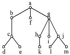
Example 20: In the rooted tree with a as a root, find the parent of c, the children of g,
the siblings of h, all ancestors of e, all descendants of b, all internal vertices, and all leaves. What is the subtree rooted at
g?
Definition : A rooted tree is called an m-ary tree if every internal vertex has no more than m children.
The tree is called a full m-ary tree if every internal vertex has exactly m children. An m-ary tree with m = 2 is called a
binary tree.
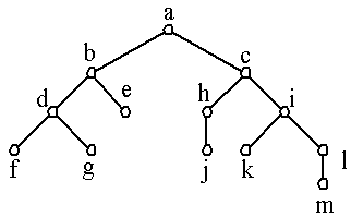
Example 21: Are the rooted trees full m-ary trees for some positive integer m?

Definition : An ordered rooted tree is a rooted tree where the children of each internal vertex are ordered. In an
ordered binary tree, if an internal vertex has two children, the first child is called the left child and the second child is called the right child.
The tree rooted at the left child is called the left subtree and the tree rooted at the right child is called the right subtree.
Example 22: What are the left and right children of d in the binary tree T (where the order is
that implied by the drawing)? What are the left and right subtrees of c?
There are numerous application of the tree. For example, the model of saturated hydrocarbons can be represented by tree
where each atom is represented by a vertex and bond is represented by an edge. The structure of organization can be represented by a tree
where each vertex represents a position in the organization and each edge represents the (direct) boss of the person of the lower position.
The structure of computer file system can be represented by tree where each directory or file is represented by a vertex and each edge represents
the containments.
Properties of trees
Theorem : A tree with n vertices has n-1 edges.
Theorem : A full m-ary tree with i internal vertices contains n = m × i + 1 vertices.
Theorem : A full m-ary tree with i = the number of internal vertices, j = the number of leaves, n
= the number of all vertices.
- n vertices has i = (n-1)/m internal vertices and j = [(m-1)n + 1]/m leaves.
- i internal vertices has n = m × i + 1 vertices and j = (m-1)i + 1 leaves.
- j leaves has n = (m × j - 1)/(m-1) vertices and i = (j-1)/(m-1)
internal vertices.
Example 23: Suppose that someone starts a chain letter. Each person who receives the letter is asked to send
it on to four other people. Some people do this, but others do not send any letters. How many people have seen the letter, including the first person,
if no one receives more than one letter and if the chain letter ends after there have been 100 people who read it but did not send it out? How many
people sent out the letter?
Definition : The level of a vertex v in a rooted tree is the length of the unique path from the root to this
vertex. The height of a rooted tree is the length of the longest path from the root to any vertex.
Example 24: Find the level of each vertex in Example 22. What is the height of this tree?
Definition : A rooted m-ary tree of height h is balanced if all leaves are at levels h or h-1.
Example 25: Which of the following tree are balanced?

Theorem : There are almost mh leaves in an m-ary tree of length h.
Corollary : If an m-ary tree of height h has l leaves, then h 
 logm l logm l  .
If the m-ary tree is full and balanced, then h = .
If the m-ary tree is full and balanced, then h =  logm l logm l
 . .
Applications of Trees
Definition : Binary search tree is a binary tree in which each vertex is labeled with a key. Moreover, vertices
that are reachable from the left subtree of a vertex v, must contain a key that is smaller than a key of the vertex v and vertices that are
reachable from the right subtree of a vertex v, must have a key that is bigger than or equal to a key of the vertex v.
Example 26: Form a binary search tree for the words: mathematics, physics, geography,
zoology, meteorology, geology, psychology and chemistry (using alphabetical order).
To maintain the binary search tree, we can use the following operations: TREE-SEARCH (searching the binary search tree for the
current key), TREE-MINIMUM (find the vertex that holds the minimum key), TREE-MAXIMUM (find the vertex that holds the maximum key),
TREE-SUCCESSOR (find the vertex that comes after the current vertex by the key value), TREE-PREDECESSOR (find the vertex that comes
before the current vertex by the key value), TREE-INSERT (insert a key into the binary search tree that maintains the binary search tree property),
TREE-DELETE (remove a vertex that holds a key from the binary search tree that maintains the binary search tree property.)
TREE-SEARCH(x, k)
INPUT : x is the current vertex and k is the key to search.
OUTPUT : pointer to the vertex that keeps k if exists, otherwise return NIL.
1. if x == NIL or k == key{x}
2.    return x
3. endif
4. if k < key{x}
5.    then return TREE-SEARCH(left{x}, k)
6.    else return TREE-SEARCH(right{x}, k)
7. endif
TREE-MINIMUM(x)
INPUT : x is the current vertex.
OUTPUT : pointer to the vertex with minimum key.
1. while left{x} != NIL
2.    x = left{x}
3. endwhile
4. return x
TREE-MAXIMUM(x)
INPUT : x is the current vertex.
OUTPUT : pointer to the vertex with maximum key.
1. while right{x} != NIL
2.    x = right{x}
3. endwhile
4. return x
TREE-SUCCESSOR(x)
INPUT : x is the current vertex.
OUTPUT : pointer to the vertex successor according to the key.
1. if right{x} != NIL
2.    then return TREE-MINIMUM(right{x})
3. endif
4. y = p{x}
5. while y != NIL and x == right{y}
6.    x = y
7.    y = p{y}
8. endwhile
9. return y
TREE-PREDECESSOR(x)
INPUT : x is the current vertex.
OUTPUT : pointer to the vertex predecessor according to the key.
1. if left{x} != NIL
2.    then return TREE-MAXIMUM(left{x})
3. endif
4. y = p{x}
5. while y != NIL and x == left{y}
6.      x = y
7.      y = p{y}
8. endwhile
9. return y
TREE-INSERT(T, z)
INPUT : T is the binary search tree, z is the key that need to be added.
OUTPUT : T is the binary search tree with z added.
1. y = NIL; x = root[T];
2. while x != NIL
3.     y = x
4.     if key{z} < key{x}
5.        then x = left{x}
6.        else x = right{x}
7.     endif
8. endwhile
9. p{z} = y
10. if y == NIL
11.    then root[T] = z
12. else if key{z} < key{y}
13.         then left{y} = z
14.      else right{y} = z
15.      endif
16. endif
To delete the key vertex from the binary search tree, we have to consider 3 cases
- if z has no child then we change the parent of z to point to NIL instead of z;
- if z has one child then we connect the parent of z to its child;
- if z has two children the we find the successor of z that does not have a left child, replace z with it and reconnect
its old place by its left child;
TREE-DELETE(T, z)
INPUT : T is a binary search tree and z is the vertex that needed to be removed.
OUTPUT : T is a binary search tree without z.
1. if left{z} == NIL or right{z}== NIL
2.    then y = z
3.    else y = TREE-SUCCESSOR(z)
4. endif
5. if left{y} != NIL then
6.    then x = left{y}
7.    else x = right{y}
8. endif
9. if x != NIL
10.    then p{x} = p{y}
11. endif
12. if p{y} == NIL
13    then root[T] = x
14    else if y == left{p{y}}
15.        then left{p{y}} = x
16.        else right{p{y}} = x
17.        endif
18. endif
19. if y != z
20.    then key{z} = key{y}
21. endif
22. return y
Definition (Prefix codes): Consider the problem of using bit strings to encode the letters of the English alphabet
(where no distinction is made between lowercase and uppercase letters). We can represent each letter with a bit string of length five, since there are
only 26 letters and there are 32 bit strings of length five. The total number of bits used to encode data is five times the number of characters in the text.
Is it possible to find a coding scheme of these letters so that, when data are coded, fewer bits are used?
The idea is to use the variable bit strings for different characters such that the letter that occurs frequently has the shorter code than the
letter that rarely occurs. In addition, the coding scheme should ensure that no bit string corresponds to more than one sequence of letters.
Codes with this property are called prefix codes.
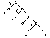
The above tree is an example of the prefix code tree with e:0, a:10, t:110, n:1110, s:1111.
Huffman code trees
Huffman code tree is used to compressing data. It uses the greedy algorithm with frequency table of occurrence of each character
to build up an optimal binary representation of each character. If we have a 100,000 character data file that we wish to compress in the table below.
| a | b | c | d | e | f |
|---|
| Frequency | 45 | 13 | 12 | 16 | 9 | 5 |
| Fixed-length |
000 | 001 | 010 | 011 | 100 | 101 |
| Variable-length |
0 | 101 | 100 | 111 | 1101 | 1100 |
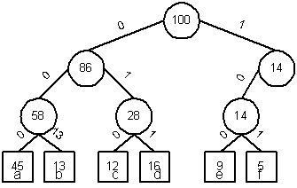 There is only six different characters appear. We are interested in designing a binary character code wherein each character is represented by
a unique binary string. If we use a fixed-length code, we need 3 bits to represent six characters: a = 000, b= 001, c = 010, d = 011, e = 100,
f = 101. This method requires 300,000 bits to code the entire file. The variable-length code can do considerably better by the following tree
representation.
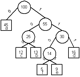
This code requires (45 + 13*3 + 12*3 + 16*3 + 9*4 + 5*4)*1000 = 224,000 bits to represent the file, a saving of approximately 25%.
Huffman code tree algorithm
The Huffman code tree algorithm constructs an optimal prefix code called a Huffman code. It builds the T corresponding to the optimal
code in a bottom-up manner. We define the frequency of each character c by f(c).
HUFFMAN-TREE(C, v)
INPUT : C is the set of characters, |C| = n and f is the frequency of each character
OUTPUT : root of the Huffman code tree.
1. n = | C |
2. Q = C used v as a keyed
3. for i = 1 to n-1 do
4.    z = ALLOCATE-NODE()
5.    x = left[z] = Extract-Min(Q)
6.    y = right[z] = Extract-Min(Q)
7.    f[z] = f[x] + f[y]
8.    Insert(Q, z)
9. endfor
10. return Extract-Min(Q)
Example 27: Find a Huffman code tree of a file that contains C = {f, e, c, b, d, a} and f(f, e, c, b, d, a) =
(5, 9, 12, 13, 16, 45).
Minimum spanning tree
Definition : Let G be a simple graph. A spanning tree of G is a subgraph of G that is a
tree containing every vertex of G.
Example 28: Find a spanning tree of the simple graphs.

Theorem : A simple graph is connected if and only if it has a spanning tree.
Definition : Two algorithms can be used to find one of the spanning tree: depth-first search and
breadth-first search.
DFS(G)
INPUT : G is a graph
OUTPUT : p the parent of each depth-first search visit
1. for each vertex u  V(G)
2. do color[v] = WHITE
3. p[u] = nil
4. endfor
5. time = 0
6. for each vertex u V(G)
2. do color[v] = WHITE
3. p[u] = nil
4. endfor
5. time = 0
6. for each vertex u  V(G)
7. do if color[u] != WHITE
8. then DFS-visit(u)
9. endif
10. endfor V(G)
7. do if color[u] != WHITE
8. then DFS-visit(u)
9. endif
10. endfor
DFS-visit(u)
INPUT : u is the node that we just visit
OUTPUT : color the appropriate node
1. color[u] = GRAY
2. d[u] = time = time + 1
3. for each v  Adj[u]
4.    do if color[v] == WHITE
5.        then p[v] = u
6.            DFS-visit(v)
7.        endif
8. endfor
9. color[u] = BLACK
10. f[u] = time = time + 1 Adj[u]
4. do if color[v] == WHITE
5. then p[v] = u
6. DFS-visit(v)
7. endif
8. endfor
9. color[u] = BLACK
10. f[u] = time = time + 1
BFS(G, s)
INPUT : G is a graph and s is the initial vertex
OUTPUT : p is the parent of visited node and d is the depth of that node.
1. for each vertex u  V(G) - {s}
2. do color[u] = WHITE
3. d[u] = V(G) - {s}
2. do color[u] = WHITE
3. d[u] =  4. p[u] = NIL
5. endfor
6. color[s] = WHITE
7. d[s] = 0
8. p[s] = NIL
9. Q = {s}
10. while (Q
   11. do u = head[Q]
12. for each v
  Adj[u]
13. do if color[v] == WHITE
14. then color[v] = GRAY
15. d[v] = d[u] + 1
16. p[v] = u
17. ENQUEUE(Q, v)
18. endif
19. endfor
20. color[u] = BLACK
21. endwhile Adj[u]
13. do if color[v] == WHITE
14. then color[v] = GRAY
15. d[v] = d[u] + 1
16. p[v] = u
17. ENQUEUE(Q, v)
18. endif
19. endfor
20. color[u] = BLACK
21. endwhile
Example 29: Find a spanning tree of the simple graphs using the depth-first search and breadth-first search
in Example 28.
Definition : A minimum spanning tree in a connected weighted graph is a spanning tree that has the
smallest possible sum of weights of its edges.
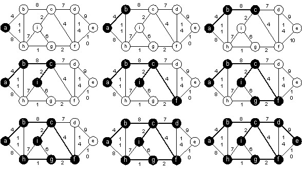
We have two different algorithms to solve this problem: Prim's algorithm and Kruskal's algorithm.
Prim's algorithm
MST-PRIM(G, w, r)
INPUT : G is an adjacency list, w is the weighted function and r is the initial vertex
OUTPUT : p is the vector parent of each vertex
1. Q = V[G]
2. for each u in Q
3.     key{u} =
4. endfor
5. key{r} = 0;
6. p{r} = NIL
7. while Q != Ø
8.     u = EXTRACT-MIN(Q)
9.     for each v in Adj[u]
10.        if v in Q and w(u, v) < key{v}
11.           then p{v} = u; key{v} =w(u, v);
12.        endif
13.    endfor
14. endwhile
15. return p
Kruskal's algorithm
MST-KRUSKAL(G, w)
INPUT : G is an adjacency list, w is a weighted function
OUTPUT : A is the set of edges in the minimum spanning tree
1. A = Ø
2. for each v in V[G]
3.     MAKE-SET(v)
4. endfor
5. sort the edges of E by nondecreasing weight w
6. for each edge (u, v) in E
7.     if FIND-SET(u) != FIND-SET(v)
8.        then A = A  {(u, v)}
9.             UNION(u, v)
10.    endif
11. endfor
12. return A {(u, v)}
9. UNION(u, v)
10. endif
11. endfor
12. return A
MAKE-SET(v)
INPUT : v is the current vertex.
OUTPUT : p is the parent of vertex v in the tree and rank is the upper bound of the length of v to a leaf.
1. p{v} = v
2. rank{v} = 0
UNION(u, v)
INPUT : u, v are vertices in the set that needed to be union using the union-by-rank heuristic.
OUTPUT : Set of the vertex from the union of u and v.
1. LINK(FIND-SET(u), FIND-SET(v))
LINK(u, v)
INPUT : u, v are vertices in the set that needed to be union using the union-by-rank heuristic.
OUTPUT : Set of the vertex from the union of u and v.
1. if rank{x} > rank{y}
2.    then p{y} = x
3.    else p{x} = y
4.         if rank{x} == rank{y}
5.         then rank{y} = rank{y} + 1
6.         endif
7. endif
FIND-SET(x)
INPUT : x is a vertex in the graph.
OUTPUT : returns the representation of the set.
1. if x != p{x}
2.    then p{x} = FIND-SET(x)
3. endif
4. return p{x}
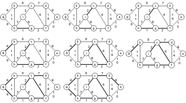
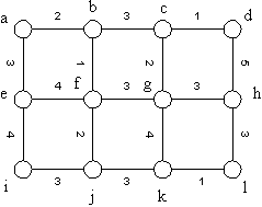
Example 29: Find the minimum spanning tree using the Prim's and Kruskal's algorithms.
|