Algorithm performance

• Q: How might we establish whether algorithm A is faster than algorithm B?
• A1: We could implement both, run them on the same input and time how long each of them takes
  Unfair test: what if one of algorithms just happens to be faster on this particular input?

Algorithm performance

• Q: How might we establish whether algorithm A is faster than algorithm B?
• A2: We could implement both, run them on lots of different inputs and time how long each of them takes on each input
  Assuming we can try every input of a particular size, this would give us best, worst and average running times for this particular implementation on this particular computer for this particular input size.
  Still an unfair test: what if one algorithm just happens to be faster on this size of input?
  What if we want a more general answer? Not tied to one computer or implementation.

Algorithm performance

• Let’s generalise things slightly … \[\mbox{The function:} T: I \rightarrow \mathbb{R}^{+}\] is a mapping from the set of all inputs $I$ to the time taken on that input.
• For any problem instance $i \in I$, $T(i)$ is the running time on $i$.
• Computing the running time for every possible problem instance is overwhelming
• Instead, group together “similar” inputs
• Gives us running time as a function of a class of instances
• How shall we group inputs?

Grouping inputs by size

Grouping inputs together of equal size is generally the most useful Bigger problems are harder to solve

• Q:What do we mean by the size of an input?
• A:It depends on the problem.
  1. Integer input → number of digits
  2. Set input → number of elements in a set
  3. Text string → number of characters
• Generally obvious
  Not always so neat: what if the input was a graph?
  May need more than one size parameter: graph size = (# vertices, # edges)

Types of performance analysis

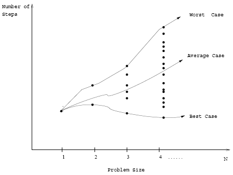
We denote the set of all instances of size $n \in \mathbb{N}$ as $I_n$.
We can define three measures of performance:

• Worst-case: \[T(n) = max\{T(i) | i \in I_n\} \] $T(n)$ = maximum time of algorithm on any input of size $n$.
• Best-case: \[T(n) = min\{T(i) | i \in I_n\} \] $T(n)$ = minimum time of algorithm on any input of size $n$.
• Average-case: \[T(n) = \frac{1}{|I_n|} \sum_{i \in I_n} T(i)\] $T(n)$ = expected time of algorithm on any input of size $n$.

Q:What assumption is being made here?
All inputs equally likely – if not we need to know the probability distribution

Type of performance analysis

We denote the set of all instances of size $n \in \mathbb{N}$ as $I_n$.
We can define three measures of performance:

Q:What is the most useful?
Q:How can we modify almost any algorithm to have a good best case running time?

Type of performance analysis

• Q: Which is most useful?
• A: Generally concentrate on worst-case execution time – strongest performance guarantee
• Q: How can we modify almost any algorithm to have a good best-case running time?
• A: Find a solution for one particular input and store it. When that input is encountered, return our precomputed answer immediately.
• Other more subtle ways of improving best-case performance.
• Best-case is generally bogus!

Measuring resource usages

Example
Summing the first $n$ positive integers:
Precondition:$n \in \mathbb{N}; Postcondition:$r$ = $\displaystyle\sum_{i = 1}^{n} i$
Two solutions and Both algorithms are correct. Which is better?

Measuring resource usage

Define some constraints:

• $i$ is the time to increment by 1
• $a$ is the time to perform an addition
• $t$ is the time to perform the loop test
• $m$ is the time to multiply two numbers
• $d$ is the time to divide by 2
• $s$ is the time to perform an assignment

Measuring resource usage

Define some constraints:

• $i$ is the time to increment by 1
• $a$ is the time to perform an addition
• $t$ is the time to perform the loop test
• $m$ is the time to multiply two numbers
• $d$ is the time to divide by 2
• $s$ is the time to perform an assignment

Measuring resource usage

Define some constraints:

• $i$ is the time to increment by 1
• $a$ is the time to perform an addition
• $t$ is the time to perform the loop test
• $m$ is the time to multiply two numbers
• $d$ is the time to divide by 2
• $s$ is the time to perform an assignment

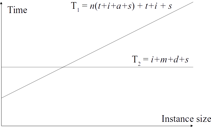
Measuring resource usage

Which is better?

Depends on size of input. Beyond intersection $T_2$ will always win.

Asymptotic Notation

• Consider $f(n)$ and $g(n)$ with integer inputs and numerical outputs
• We say $f$ grows no faster then $g$ in the limit if:
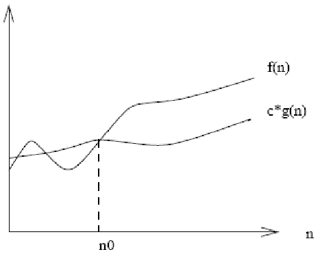
  There exist positive constants $c$ and $n_0$ such that $f(n) \leq c g(n)$ for all $n > n_0$
• We write this as: \[f(n) = O(g(n))\] and read “f is Big Oh of g” or “f is asymptotically dominated by g” or “g is an upper bound on f” or “f grows no faster than g”

Asymptotic Notation

Definition of Big Oh

• Formal definition: \[f(n) = O(g(n)) \mbox{ iff } \exists c \in \mathbb{R}^{+} \exists n_0 \in \mathbb{N} \forall n > n_0, f(n) \leq c g(n)\]
• Breaking this up:
  $n_0$ that $n > n_0$ means we don't care about small $n$.
  $c, f(n) \leq c g(n)$ means we don't care about constant speedups.
  Unusual notation: “one way equality”
  Really an ordering relation (think of < and >)
  $f(n) = O(g(n))$ definitely does not imply $g(n) = O(f(n))$

Definition of Big Oh

• Might like to think in terms of sets: \[O(g(n)) = \{f(n) | \exists c \in \mathbb{R}^{+} \exists n_0 \in \mathbb{N} \forall n > n_0, f(n) \leq c g(n)\}\]
• In this way:we can interpret $f(n) = O(g(n))$ as $f(n) \in O(g(n))$.

Big Oh example

• \[ n^2 + 1 = O(n^2) \mbox{ --- True or False?}\] How would we prove it?
• Consider the definition: \[ f(n) = O(g(n)) \mbox{ iff } \exists c \in \mathbb{R}^{+} \exists n_0 \in \mathbb{N} \forall n > n_0, f(n) \leq c g(n)\]
• To prove $\exists x, P$ we need: (1) A witness (value) for $x$ (2) A proof that $P$ holds when witness substituted for $x$.

Big Oh example

• Need to find an $n_0$ such that $\forall n > n_0, n^2 + 1 < 2 n^2$
• In this case, $n_0$ = 1 or greater value will do.
• By convention, always complex to simple: complex form = O(simple form) \[\begin{array}{lcl} 3 n^2 + 102 n + 56 & = & O(n^2) \\ 3 n^2 + 102 n + 56 & = & O(n^3) \\ 3 n^2 + 102 n + 56 & = & O(n) \end{array}\] Related operators follow from definition of Big Oh…

Definition of Big Omega

• If Big Oh is like $\leq$ then Big Omega is like $\geq$ \[ f(n) = \Omega(g(n)) \mbox{ iff } g(n) = O(f(n))\] “f grows no slower than g” or Read as “f is Big Omega of g”
• Express as a set: \[ \Omega(g(n)) = \{f(n) | \exists c \in \mathbb{R}^{+} \exists n_0 \in \mathbb{N} \forall n > n_0, f(n) \geq c g(n)\}\] \[\begin{array}{lcl} 3 n^2 + 102 n + 56 & = & \Omega(n^2) \\ 3 n^2 + 102 n + 56 & = & \Omega(n^3) \\ 3 n^2 + 102 n + 56 & = & \Omega(n) \end{array}\]

Graph of Big Omega

Definition of Theta

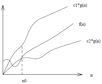
• Theta is like = \[f(n) = \theta(g(n)) \mbox{ iff } f(n) = O(g(n)) \mbox{ and } f(n) = \Omega(g(n))\] “f grows at the same rate as g” or “f is theta of g”
• Express as a set: \[\theta(g(n)) = O(g(n)) \cap \Omega(g(n)) \] \[\begin{array}{lcl} 3 n^2 + 102 n + 56 & = & \theta(n^2) \\ 3 n^2 + 102 n + 56 & = & \theta(n^3) \\ 3 n^2 + 102 n + 56 & = & \theta(n) \end{array}\]

Graph of Theta