Lecture 3:Computation
Written byKrung Sinapiromsaran
July 2557
Outline
- Asymptotic notations and their relationships
- Asymptotic dominance
- The power of efficient algorithms
- Logarithms in algorithm analysis
- Binary search
- Basic algorithm analysis
- Recursive algorithms
- Limits of computation
- Complexity of a problem
Objective
- To be able to prove relationships among asymptotic notations
- Can apply the technique to analyze any algorithms
- Explain the logarithm terms that appear in the analysis
- Can analyze iterative and recursive algorithms.
- Can show the complexity class of any given problems
Summary
\[\begin{array}{clcl} \leq & f(n) = O(g(n)) & \mbox{iff} & \exists c \in \mathbb{R}^{+} \exists n_0 \in \mathbb{N} \forall n > n_0, f(n) \leq c g(n) \\ \geq & f(n) = \Omega(g(n)) & \mbox{iff} & g(n) = O(f(n)) \\ = & f(n) = \theta(g(n)) & \mbox{iff} & f(n) = O(g(n)) \mbox{ and } g(n) = O(f(n)) \\ < & f(n) = o(g(n)) & \mbox{iff} & f(n) = O(g(n)) \mbox{ and } f(n) \neq \theta(g(n)) \\ > & f(n) = \omega(g(n)) & \mbox{iff} & f(n) = \Omega(g(n)) \mbox{ and } f(n) \neq \theta(g(n)) \end{array}\]Further complexity rules
- Big Oh is reflexive: $f(n) = O(f(n))$
Prove by setting $c$ = 1 and $n_0$ = 0 - Big Oh is transitive: $f(n) = O(g(n))$ and $g(n) = O(h(n)) \rightarrow f(n) = O(h(n))$
Determine $c$ and $n_0$ that makes this work! - Drop low order term: \[f(n) = O(g(n)) \rightarrow f(n) + g(n) = \theta(g(n))\]
- Drop the leading constant: \[f(n) = O(g(n)) \mbox{ and } h(n) = O(k(n)) \rightarrow f(n) \times h(n) = O(g(n) \times k(n))\]
- Generally, \[\sum_{i = 0}^{k} a_i n^i = \theta(n^k)\]
Further complexity rules
- Two useful rules for logarithms: 1 = $n^0$ = $o(\log n)$, $\log n$ = $o(n^r)$ for all positive $r$. So $\log n$ lies somewhere between constant time and $n^r$ for any $r$.
Asymptotic Dominance
Recall \[\begin{array}{lcl} f(n) = o(g(n)) & \mbox{iff} & \lim_{n \rightarrow \infty} \frac{f(n)}{g(n)} = 0 \\ f(n) = \omega(g(n)) & \mbox{iff} & \lim_{n \rightarrow \infty} \frac{f(n)}{g(n)} = \infty \\ f(n) = \theta(g(n)) & \mbox{iff} & \lim_{n \rightarrow \infty} \frac{f(n)}{g(n)} = r > 0 \end{array}\]
- We say $f(n)$ dominates $g(n)$, written $f(n) >> g(n)$ if $g(n) = O(f(n))$ We can therefore state a dominance ranking of complexity classes which commonly arise in algorithm analysis: \[n^n >> n! >> 2^n >> n^3 >> n^2 >> n \log n >> n >> \log n >> 1\] You must remember these – listing them in order should be second nature
Asymptotic Dominance
Including some more obsecure classes of complexity \[\begin{array}{l} n^n >> n! >> c^n >> n^3 >> n^2 >> n^{1+\varepsilon} >> \\ n \log n >> n >> \sqrt{n} >> \log^2 n >> \log n >> \\ \frac{\log n}{\log\log n} >> \log\log n >> \alpha(n) >> 1\end{array}\]
Common asymptotic class
| Name | $T = f(n)$ |
|---|---|
| Constant | 1 |
| Logarithmic | $\log n$ |
| Linear | $n$ |
| Log-linear (or linearithmic) | $n \log n$ |
| Quadratic | $n^2$ |
| Cubic | $n^3$ |
| Polynomial | $n^k$ |
| Exponential | $b^n$ |
Asymptotic Dominance in Action
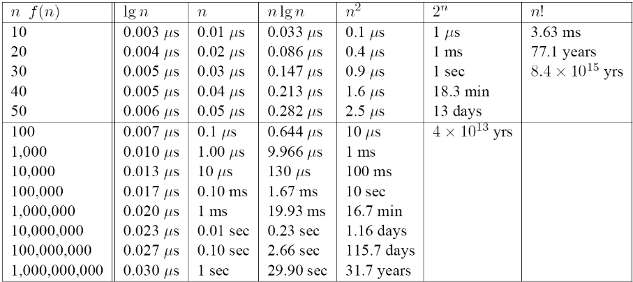
On a computer executing 1 instruction per nanosecond, running time for varying input size:
The big match up...
IBM Roadrunner $1.026$ quadrillion calculations per second ($1.026 \times 10^15$) Running an Ο($n^2$) algorithm

The big match up...
2.3 million times slower, stacked on top of each other would be 27km high!
But we’re going to beat Roadrunner with one iPhone using a better algorithm,
Apple iPhone 450 million calculations per second Running an Ο($n \log n$) algorithm

The big match up...
| No. items | iPhone | Roadrunner |
|---|---|---|
| 1 million | 0.03 sec. | 0.0009 sec. |
| 100 million | 4.1 sec. | 9.75 sec. |
| 1000 million | 46 sec. | 974 sec. |
Implications of Asymptotic Dominance
- Exponential algorithms are hopeless for anything beyond very small inputs
- Quadratic algorithms are hopeless beyond about one million
- O($n \log n$) is possible to about one billion
- O($\log n$) never struggles
- Logarithmic time algorithms grow remarkably slowly
- Logs crop up often in algorithm analysis
Logarithm in Algorithm analysis
- Note that \[b^x = y \mbox{ means } x = \log_b y\] Or equivalently, \[b^{\log_b y} = y\] Logarithms arise whenever we repeatedly halve something
- Recall: $\log_a (x y) = \log_a (x) + \log_a (y)$ and $\log_b (a)$ = $\displaystyle\frac{\log_c a}{\log_c b}$
- The base doesn’t matter in asymptotic analysis
- Changing from base $a$ to $c$ is just multiplying by a constant: \[\log_a b = K log_c b \mbox{ where } K = \frac{1}{\log_c a}\]
Binary Search
- Binary search is a very useful method for searching an ordered list
Given an array: a[1:n] where $a[1] \leq a[2] \leq ... \leq a[n]$ - We wish to find the element $x$ in the list
i.e. we require the index: $i$ where $a[i-1] < x \leq a[i]$ - Q: Why can’t we just look for $a[i] = x$?
- Strategy:
- Examine element $a[m]$ where $\displaystyle m = \frac{n}{2}$
- If $x = a[m]$, stop – we’re done
- If $x > a[m]$, then throw away bottom half of list, recursively search remaining half, otherwise vice versa
Binary Search
- For each comparison, we half the number of potential items
- Q: Complexity of binary search (number of comparisons):
- Best case?
- We find it at the middle element: $T(n) = \theta(1)$
- Worst case?
- We have to keep halving the search space until only one item remains: $T(n) = \theta(\log(n))$
- Implications:
Find any name in the Manhattan phone book (1 million names) in 20 comparisons - Never lose at “20 questions” again – binary search the dictionary
Basic Algorithm Analysis
- To summarize, our simplifications are:
- Real computer to RAM model
- Running time measured by number of instructions
- Group inputs by size and focus on worst case
- Asymptotic analysis ignores constant factors/low order terms
- Result of these is that asymptotic complexity can be found directly from pseudocode
- Employ some simple rules for worst case analysis of simple structures
Basic Algorithm Analysis
- Sequenced statements:
- If $T(I_i)$ is worst-case execution time of statement $I_i$, then for sequenced statements: \[T(I_1; I_2) = T(I_1) + T(I_2)\]
Basic Algorithm Analysis
- Choice statements:
- So we can’t get an exact answer → we can’t say for certain what $T(I)$ will equal
- Q: Suggestions?
- We’re interested in worst case, so we take the slowest
- Because answer is inexact we use Big Oh, we’re saying running time is bounded from above by this worst case time: \[T(\mbox{If } C \mbox{ then } I_1 \mbox{ else } I_2) = O(T(C) + max\{T(I_1), T(I_2)\})\]
Basic Algorithm Analysis
- Iteration statements:
- Q: What information are we missing to give an answer?
- We need to know how many times the loop will iterate Assuming we know this (= $n$), time is: \[T(\mbox{while } C \mbox{ do } I) = O \left(\sum_{i = 1}^{n} T(C) + T(I) \right)\]
- Iteration statements (loops) are more complex than sequential or choice
- Require use of sums
Algorithm analysis example
- Analyse running time as function of $n$.
- Q: How many times do we increment s? What is the asymptotic complexity?
- Example 1
- We go round the loop $n$ times, so $s$ is incremented $n$ times: $f(n) = \theta(n)$
- Expressed as a sum: $\displaystyle\sum_{i = 1}^{n} 1 = n$
Algorithm analysis example
- Analyse running time as function of n
- Q: How many times do we increment s? What is the asymptotic complexity?
- Example 2
- Same as before the inner for-loop: $\displaystyle\sum_{j = 1}^{n} 1 = n$
- The outer for-loop: $\displaystyle\sum_{i = 1}^{n} n = n^2$ and complexity is: $f(n) = \theta(n^2)$
Analyze running time
- Q: How many times do we increment $s$? What is the asymptotic complexity?
- Example 3
- Same as before the inner for-loop: $\displaystyle\sum_{j = 1}^{i} 1 = i$
- The outer for-loop: $\displaystyle\sum_{i = 1}^{n} i = \frac{n(n+1)}{2}$.
- We do less work than before, however, the asymptotically two algorithms have the same running time: $f(n) = \theta(n^2)$
Tower of Hanoi
Move $n$ discs from A to B using C as a spare observing following rules:
- Only one disc can be moved at a time
- Discs can only be placed on top of larger discs

Recursive Algorithm:Classic example
- To move $n$ discs from A to B:
- First move $n-1$ discs from A to C, then move 1 from A to B, finally move $n-1$ discs back to B

Tower of Hanoi recursive algorithm
- From our example, we would call function with: ToH(8,A,B,C)
- If we measure time in terms of how many moves we have to make. What is $T(n)$?
- Base case is T(1) = 1, in general $\displaystyle T(n) = \left\{\begin{array}{ll} 1 & \mbox{ if } n = 1 \\ 2 T(n-1) + 1 & \mbox{ if } n > 1\end{array}\right.$
Tower of Hanoi analysis
\[T(n) = \left\{\begin{array}{ll} 1 & \mbox{ if } n = 1 \\ 2 T(n-1) + 1 & \mbox{ if } n > 1\end{array}\right.\]- No standard method for solving recurrences
- Can learn some tricks
- In general, make informed guess at solution and prove using induction
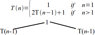
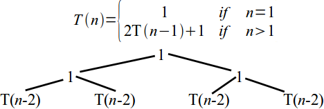
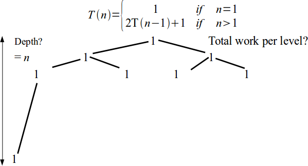
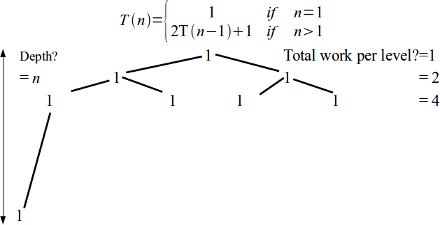
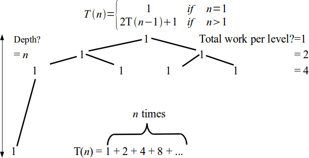
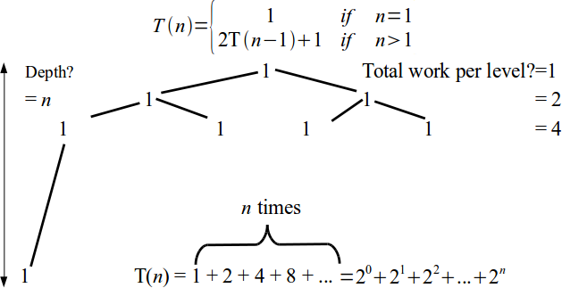
- An intuitive approach is a recursion tree.
Recursive Algorithm Analysis
\[T(n) = \left\{\begin{array}{ll} 1 & \mbox{ if } n = 1 \\ 2 T(n-1) + 1 & \mbox{ if } n > 1\end{array}\right.\]T(n)
Recursive Algorithm Analysis
Recursive Algorithm Analysis
Recursive Algorithm Analysis
Recursive Algorithm Analysis
Recursive Algorithm Analysis
Recursive Algorithm Analysis
Recursive Algorithm Analysis
\[T(n) = \left\{\begin{array}{ll} 1 & \mbox{ if } n = 1 \\ 2 T(n-1) + 1 & \mbox{ if } n > 1\end{array}\right. = \sum_{i = 0}^{n} 2^i\]- The standard identity for geometric series with the ratio $r$ is $\displaystyle\sum_{i = 0}^{n} r^i = \frac{1 - r^{n+1}}{1 - r}.$
- Hence, Tower of Hanoi is exponential complexity: $T(n) = \theta(2^n)$.
Computational class and feasiblity
| Name | $T = f(n)$ |
|---|---|
| Constant | 1 |
| Logarithmic | $\log n$ |
| Linear | $n$ |
| Log-linear (or linearithmic) | $n \log n$ |
| Quadratic | $n^2$ |
| Cubic | $n^3$ |
| Polynomial | $n^k$ |
| Exponential | $b^n$ |
Q: Where do we draw the line? What is an “efficient” algorithm?
Is there a limit to what we can consider feasible?
Polynomial time algorithm
- This decision is somewhat arbitrary
- We equate an efficient algorithm with one which runs in polynomial time \[T(n) = O(p(n)) \mbox{ and } \exists k \in \mathbb{N}, p(n) = O(n^k)\]
- We call an algorithm with running time $T(n)$ is a polynomial-time algorithm.
Complexity of a problem
- We’ve been thinking about the complexity of an algorithm
Q: What might we mean by the complexity of a problem?
A: Lowest worst-case complexity of any algorithm that can solve it - Arguing exact complexity is sometimes difficult
- We may only be able to give lower bounds (examples later)
- We can now talk about “polynomial-time solvable” problems
...meaning: there is a polynomial-time algorithm that can solve the problem - For many important problems there is no known efficient algorithm.
Examples of hard problems
- The shortest path problem for a robot arm we saw in Lecture 1 is commonly known as the “Travelling Salesman Problem”
- Huge implications for logistics if it could be solved
- Knapsack problem: given a set of items, each with a weight and value, can a value of at least $V$ be achieved without exceeding the weight $W$?
- These problems are easy to explain, easy to verify that a solution is correct, but extremely difficult to solve
- For anything but trivial problems, computation time is astronomical.
- There is a class of such problems which are all equivalent (solve one = solve all)
- They are known as NP-complete problems.
NP-complete problems
- NP stands for Nondeterministic Polynomial time
- NP-complete problems have two properties:
- Any given solution to the problem can be verified in polynomial time
- If the problem can be solved in polynomial time, so can every problem in NP
- At present, establishing your problem is NP-complete means don’t bother trying to solve it exactly
- One of the great problems in computer science is to establish whether a polynomial time algorithm can be found to solve an NP-complete problem
- Although it is thought unlikely that P = NP (since no-one has found such an algorithm yet) it also not been proven that P ≠ NP
P = NP?
Solve “P = NP?” and EARN $\$1,000,000$
- This is such an important problem that the Clay Mathematics Institute has offered a one million dollar prize for its solution.
Show that P = NP and EARN $\$7,000,000$ - Some people think that if P = NP it may be possible for computers to “find a formal proof of any theorem which has a proof of a reasonable length”
- It is therefore likely that you could use a computer to solve the other 6 CMI prize problems and claim all of the prize money
- Get working on it!
Conclusion
- We now have a set of tools to compare algorithms:
- We know how to go from pseudocode to algorithm complexity
- Logarithmic time algorithms arise from divide-and-conquer - very efficient and can be powerful
- We know how to compare complexities and when to say “too slow!”
Comments and Suggestions
- Assistant Professor Krung Sinapiromsaran
- Web: http://pioneer.netserv.chula.ac.th/~skrung
- Email: Krung.S@chula.ac.th
